Guide chapters

Colours and spatial maps

Colour fields change appearance; density and scale fields change where nodes fit. Keep those roles separate when interpreting a map.

Colour schemes

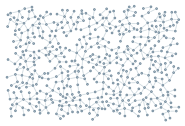
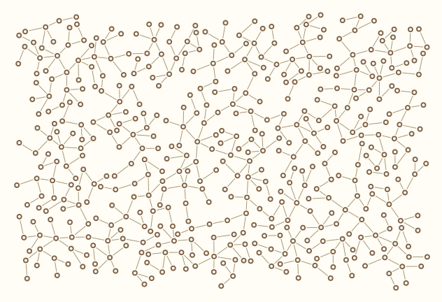
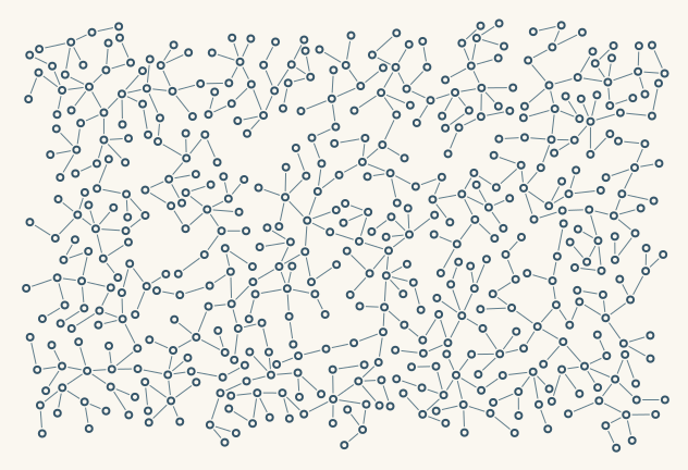
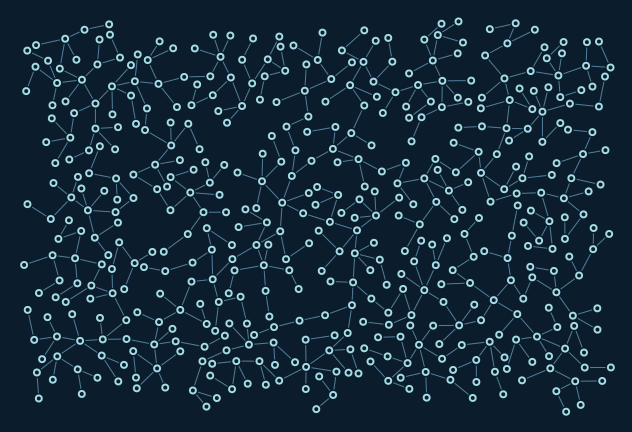
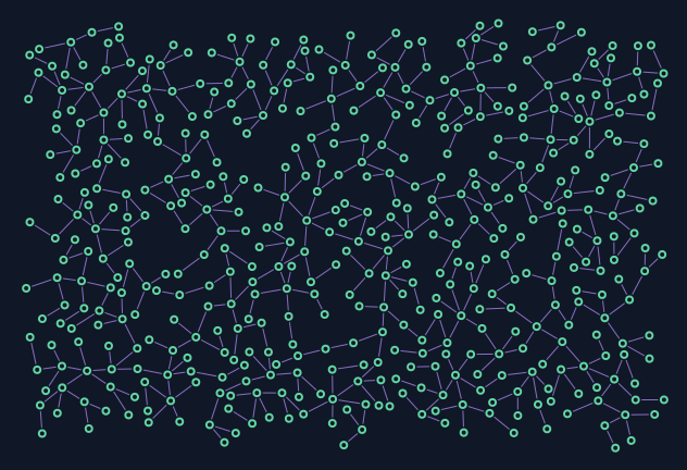
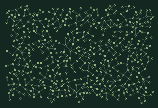
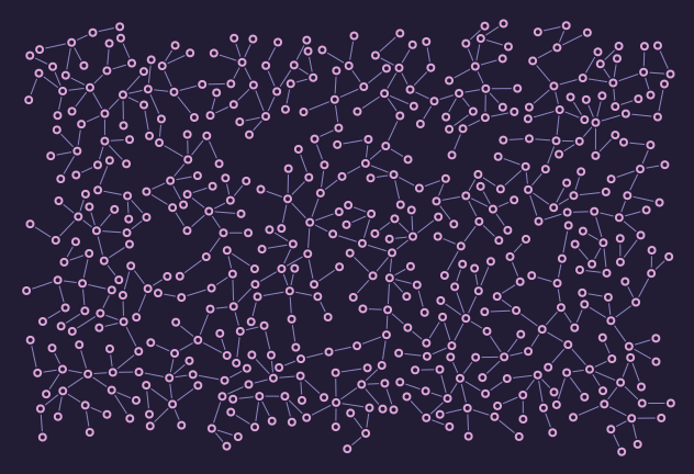
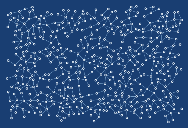
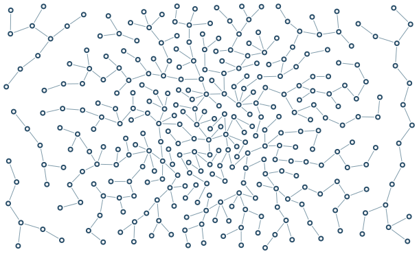
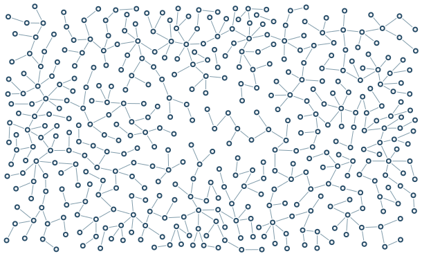
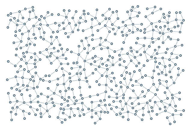
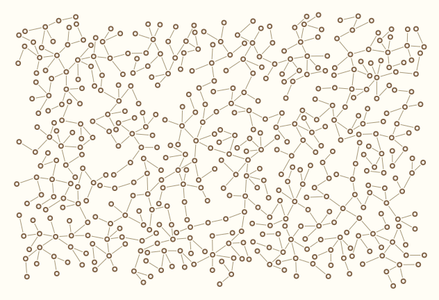
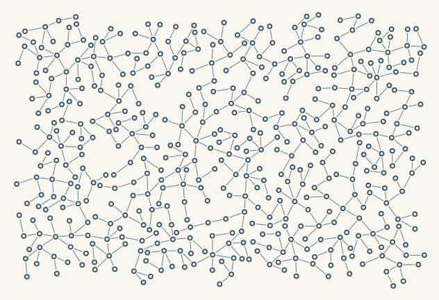
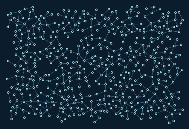
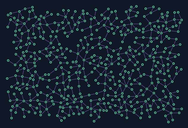
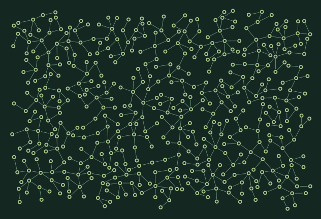
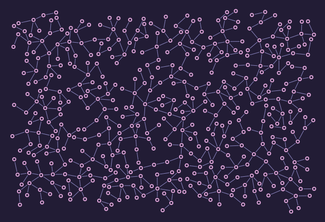
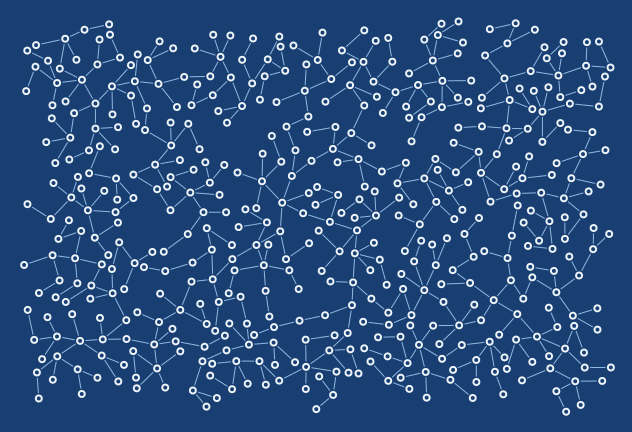
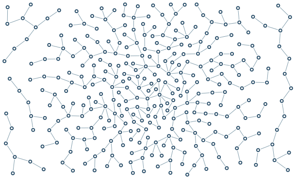
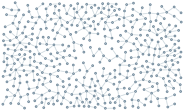
Porcelain is white; Linen and Light are warm near-white alternatives. Arctic is a dark blue ice palette.

Palette Porcelain

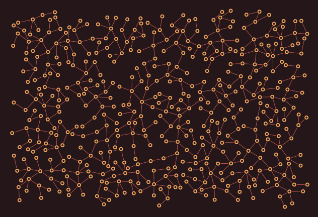
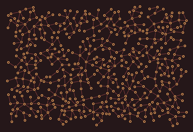
Only the colour scheme changes here; no text means the exact same geometry.

632 × 432; 480 nodes

Reproduce / SVG

graph-ics render --example sprawl --palette porcelain --nodes 480 --seed 7 --node-shape circle --edge-style solid --scale 1 --margin 16 --output examples/output/palette-porcelain.png

SVG

Palette Linen

Only the colour scheme changes here; no text means the exact same geometry.

632 × 432; 480 nodes

Reproduce / SVG

graph-ics render --example sprawl --palette linen --nodes 480 --seed 7 --node-shape circle --edge-style solid --scale 1 --margin 16 --output examples/output/palette-linen.png

SVG

Palette Historical

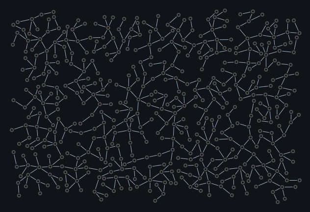
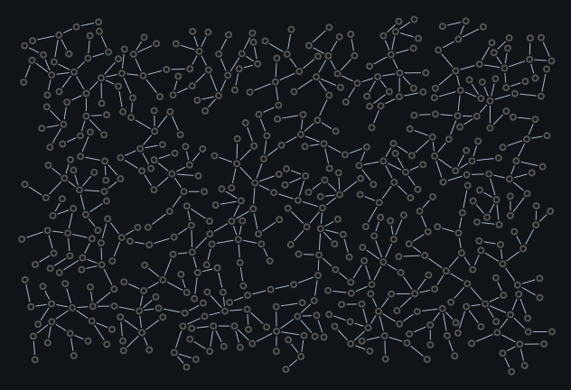
Only the colour scheme changes here; no text means the exact same geometry.

632 × 432; 480 nodes

Reproduce / SVG

graph-ics render --example sprawl --palette historical --nodes 480 --seed 7 --node-shape circle --edge-style solid --scale 1 --margin 16 --output examples/output/palette-historical.png

SVG

Palette Light

Only the colour scheme changes here; no text means the exact same geometry.

632 × 432; 480 nodes

Reproduce / SVG

graph-ics render --example sprawl --palette light --nodes 480 --seed 7 --node-shape circle --edge-style solid --scale 1 --margin 16 --output examples/output/palette-light.png

SVG

Palette Arctic

Only the colour scheme changes here; no text means the exact same geometry.

632 × 432; 480 nodes

Reproduce / SVG

graph-ics render --example sprawl --palette arctic --nodes 480 --seed 7 --node-shape circle --edge-style solid --scale 1 --margin 16 --output examples/output/palette-arctic.png

SVG

Palette Aurora

Only the colour scheme changes here; no text means the exact same geometry.

632 × 432; 480 nodes

Reproduce / SVG

graph-ics render --example sprawl --palette aurora --nodes 480 --seed 7 --node-shape circle --edge-style solid --scale 1 --margin 16 --output examples/output/palette-aurora.png

SVG

Palette Ember

Only the colour scheme changes here; no text means the exact same geometry.

632 × 432; 480 nodes

Reproduce / SVG

graph-ics render --example sprawl --palette ember --nodes 480 --seed 7 --node-shape circle --edge-style solid --scale 1 --margin 16 --output examples/output/palette-ember.png

SVG

Palette Forest

Only the colour scheme changes here; no text means the exact same geometry.

632 × 432; 480 nodes

Reproduce / SVG

graph-ics render --example sprawl --palette forest --nodes 480 --seed 7 --node-shape circle --edge-style solid --scale 1 --margin 16 --output examples/output/palette-forest.png

SVG

Palette Orchid

Only the colour scheme changes here; no text means the exact same geometry.

632 × 432; 480 nodes

Reproduce / SVG

graph-ics render --example sprawl --palette orchid --nodes 480 --seed 7 --node-shape circle --edge-style solid --scale 1 --margin 16 --output examples/output/palette-orchid.png

SVG

Palette Blueprint

Only the colour scheme changes here; no text means the exact same geometry.

632 × 432; 480 nodes

Reproduce / SVG

graph-ics render --example sprawl --palette blueprint --nodes 480 --seed 7 --node-shape circle --edge-style solid --scale 1 --margin 16 --output examples/output/palette-blueprint.png

SVG

Colour, density and scale

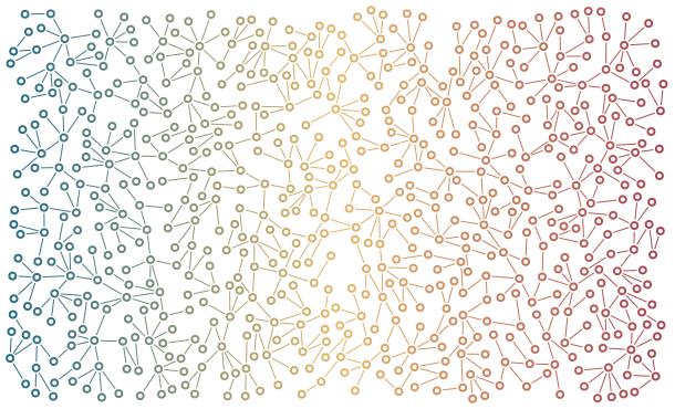
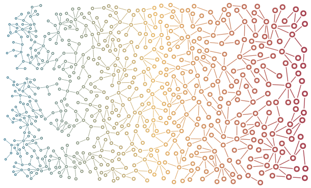
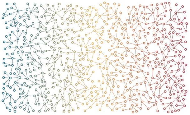
Colour Gradient

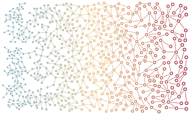
A continuous colour field, sampled at node centres and edge midpoints. It does not alter geometry.

650 nodes of 650 requested. Stop: target_reached. 240/240 occupied tiles; 100.0% of tile area has a node. This is a coarse coverage measure, not solid ink coverage.

JSON scene · YAML scene · SVG

Settings and command

graph-ics render --config docs/scenes/colour-gradient.yaml --output examples/output/colour-gradient.png

{
  "version": 1,
  "palette": "porcelain",
  "width": 600,
  "height": 360,
  "nodes": 650,
  "seed": 7,
  "growth": {
    "total_attempts": 35000,
    "refill_passes": 2,
    "coverage": {
      "tile_size": 30,
      "reseed_attempts": 1200
    }
  },
  "color_map": {
    "field": {
      "kind": "gradient",
      "axis": "x"
    },
    "colors": [
      "#246b87",
      "#e7b96d",
      "#a64152"
    ]
  }
}

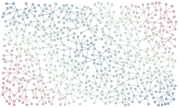
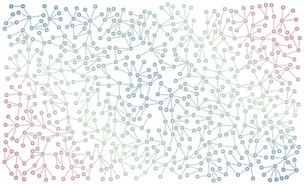
Colour Raster

A painted scalar raster becomes a colour map through bilinear interpolation.

650 nodes of 650 requested. Stop: target_reached. 240/240 occupied tiles; 100.0% of tile area has a node. This is a coarse coverage measure, not solid ink coverage.

JSON scene · YAML scene · SVG

Settings and command

graph-ics render --config docs/scenes/colour-raster.yaml --output examples/output/colour-raster.png

{
  "version": 1,
  "palette": "porcelain",
  "width": 600,
  "height": 360,
  "nodes": 650,
  "seed": 7,
  "growth": {
    "total_attempts": 35000,
    "refill_passes": 2,
    "coverage": {
      "tile_size": 30,
      "reseed_attempts": 1200
    }
  },
  "color_map": {
    "field": {
      "kind": "raster",
      "pixels": [
        [0, 0.4, 1],
        [0.8, 0.2, 0.7],
        [1, 0.5, 0]
      ]
    },
    "colors": [
      "#274f7c",
      "#a7c6ad",
      "#b34d6a"
    ]
  }
}

Radial Density

An abstract focal point, not population: density rises smoothly toward the centre.

321 nodes of 650 requested. Stop: attempt_budget_exhausted. 212/240 occupied tiles; 88.3% of tile area has a node. This is a coarse coverage measure, not solid ink coverage.

JSON scene · YAML scene · SVG

Settings and command

graph-ics render --config docs/scenes/radial-density.yaml --output examples/output/radial-density.png

{
  "version": 1,
  "palette": "porcelain",
  "width": 600,
  "height": 360,
  "nodes": 650,
  "seed": 7,
  "growth": {
    "total_attempts": 35000,
    "refill_passes": 2,
    "coverage": {
      "tile_size": 30,
      "reseed_attempts": 1200
    }
  },
  "fields": {
    "density": {
      "kind": "radial",
      "min": 0.0008,
      "max": 0.006,
      "sigma": 110
    }
  }
}

Painted Density

A coarse painted mask creates bands of dense and open texture. Any scalar measurement can play this role.

420 nodes of 650 requested. Stop: attempt_budget_exhausted. 236/240 occupied tiles; 98.3% of tile area has a node. This is a coarse coverage measure, not solid ink coverage.

JSON scene · YAML scene · SVG

Settings and command

graph-ics render --config docs/scenes/painted-density.yaml --output examples/output/painted-density.png

{
  "version": 1,
  "palette": "porcelain",
  "width": 600,
  "height": 360,
  "nodes": 650,
  "seed": 7,
  "growth": {
    "total_attempts": 35000,
    "refill_passes": 2,
    "coverage": {
      "tile_size": 30,
      "reseed_attempts": 1200
    }
  },
  "fields": {
    "density": {
      "kind": "raster",
      "pixels": [
        [0.001, 0.006, 0.001],
        [0.006, 0.001, 0.006],
        [0.001, 0.006, 0.001]
      ]
    }
  }
}

Variable Dimensions

Coordinated scale changes radius, wall, gap, line width and length together; colour remains independent.

650 nodes of 650 requested. Stop: target_reached. 238/240 occupied tiles; 99.2% of tile area has a node. This is a coarse coverage measure, not solid ink coverage.

JSON scene · YAML scene · SVG

Settings and command

graph-ics render --config docs/scenes/variable-dimensions.yaml --output examples/output/variable-dimensions.png

{
  "version": 1,
  "palette": "porcelain",
  "width": 600,
  "height": 360,
  "nodes": 650,
  "seed": 7,
  "growth": {
    "total_attempts": 35000,
    "refill_passes": 2,
    "coverage": {
      "tile_size": 30,
      "reseed_attempts": 1200
    }
  },
  "fields": {
    "coordinated_scale": {
      "kind": "gradient",
      "min": 0.55,
      "max": 1.5
    }
  },
  "color_map": {
    "field": {
      "kind": "gradient",
      "axis": "x"
    },
    "colors": [
      "#246b87",
      "#e7b96d",
      "#a64152"
    ]
  }
}

Population as one possible input

The UK and Spain examples use bundled population estimates. Other scalar measurements or painted fields work too. These maps are illustrative transformations, not one node per person.

Data-driven growth

The shape of a population.

UK population-density estimates guide a network inside the country boundary. Cities become finer and denser; rural areas leave more breathing room.

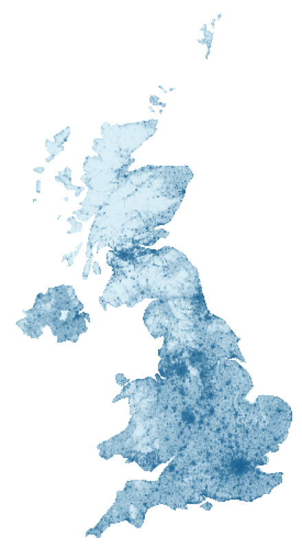
WorldPop 2020 population density across the UK — Input: 2020 estimates, persons per square kilometre. Pale blue is near zero; dark blue is 10,000 or more. The colour scale is logarithmic.

UK density-guided graph — Output: a density-guided graph. Open the image for its full resolution. Nodes do not represent individual people.

Make this example

graph-ics render --example uk_population --palette porcelain --output examples/output/uk.png

The input is bundled with the library and runs offline. It includes Northern Ireland and UK islands, and excludes the Republic of Ireland. Small islands and narrow coastal features may remain empty.

From density to spacing

Population spans a wide range. A logarithmic mapping compresses the extremes so city structure remains readable: t = min(1, log(1+density)/log(10001)). Preferred spacing is 5 + 20*(1-t); geometry scale is 0.45 + 0.9*(1-t). Cities receive smaller, closer nodes. Collision checks and finite attempt budgets still limit packing.

This is an artistic transformation, not a linear population map. The source raster is resampled from approximately 1 km to 360 by 560 cells. The boundary is simplified; no-data samples become zero. Pixel centres share the boundary projection: longitude scaled by cos(55 degrees), north at the top. This display projection is not equal-area.

Different uses of the same map

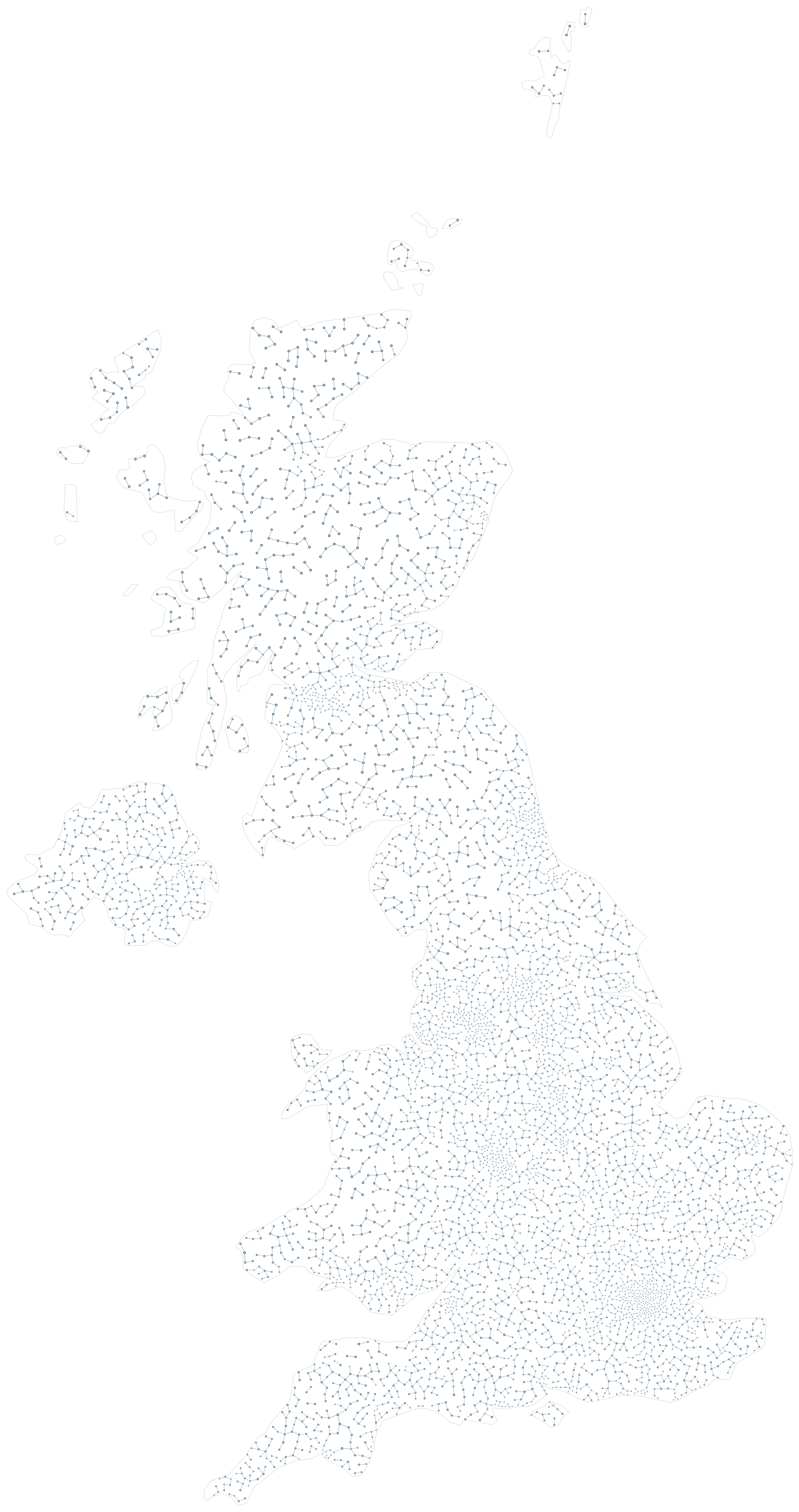
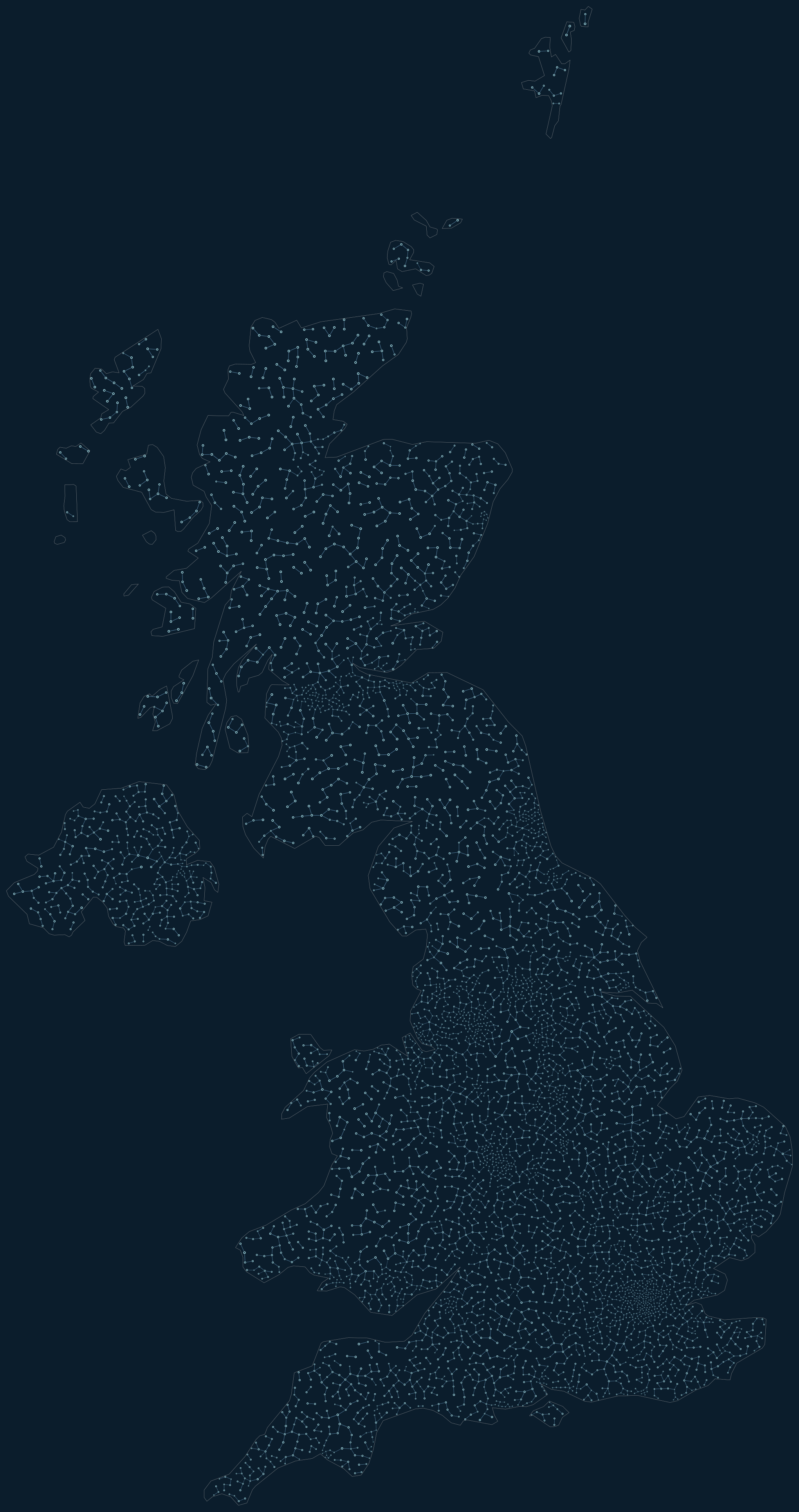
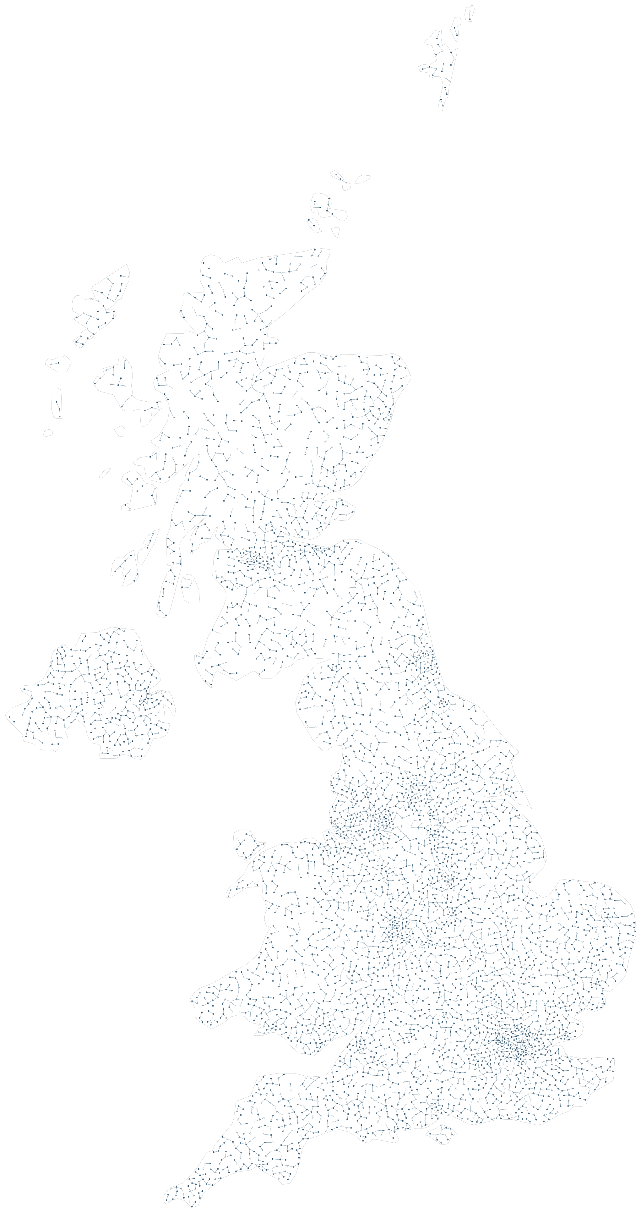
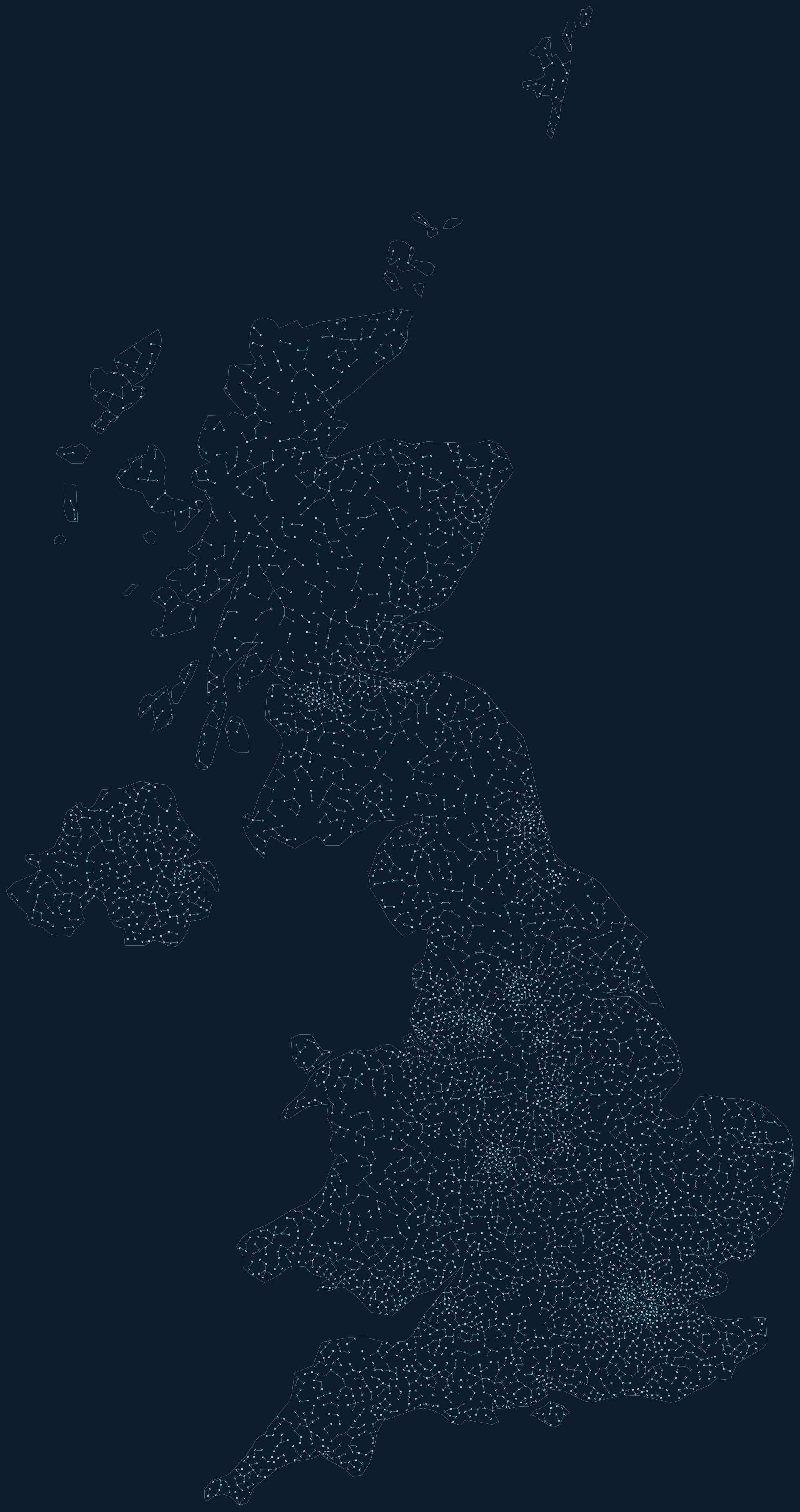
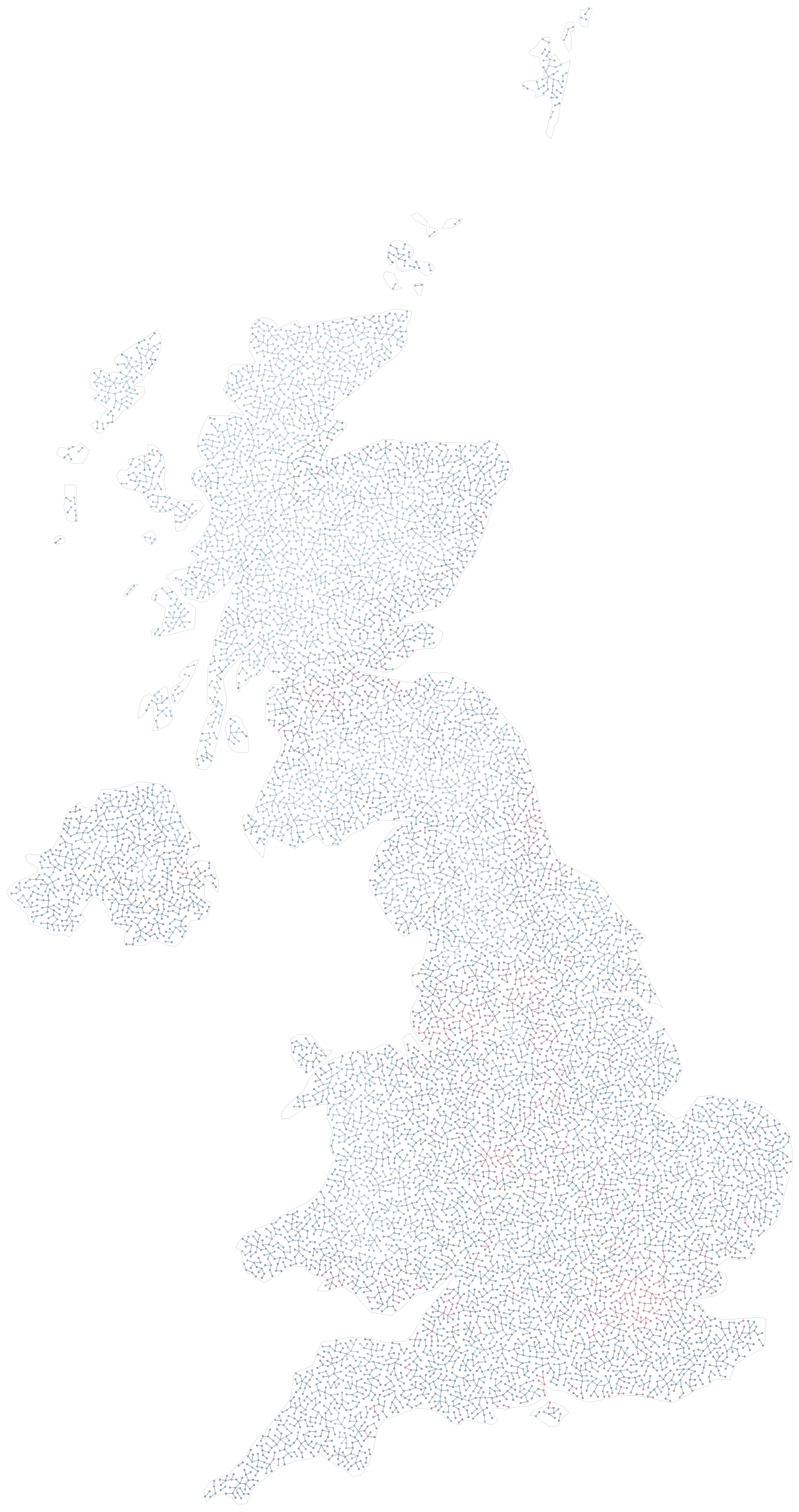
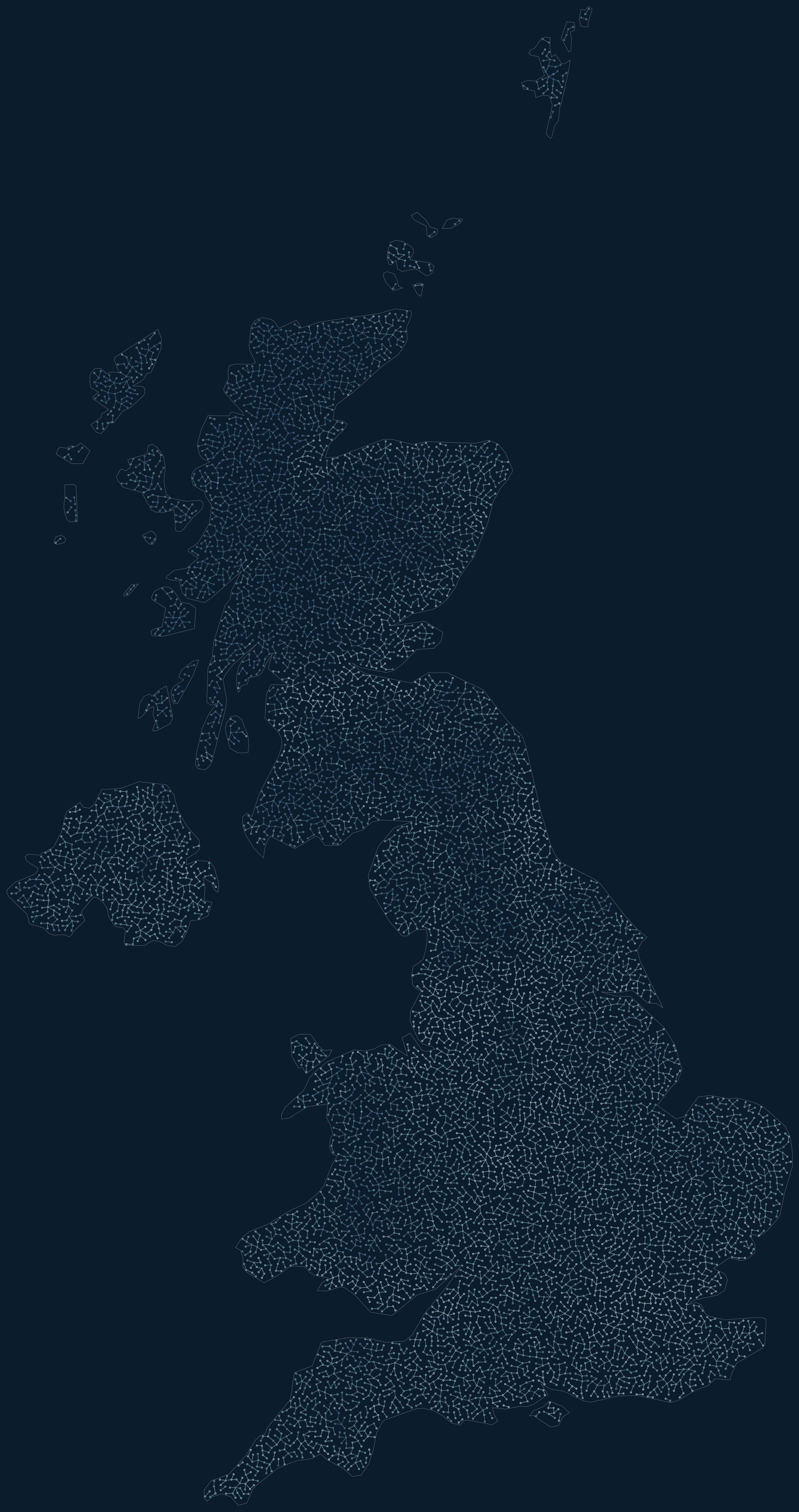
Population is just one scalar input. Compare spacing-only, colour-only, and coordinated size/spacing below. The scene guide also demonstrates abstract radial fields and painted rasters, suitable for visual emphasis or any other spatial measurement.

UK: size and spacing / porcelain

graph-ics render --example uk_population --palette porcelain --output examples/output/uk_population-porcelain.png

UK: size and spacing / arctic

graph-ics render --example uk_population --palette arctic --output examples/output/uk_population-arctic.png

UK: spacing only / porcelain

graph-ics render --example uk_density_only --palette porcelain --output examples/output/uk_density_only-porcelain.png

UK: spacing only / arctic

graph-ics render --example uk_density_only --palette arctic --output examples/output/uk_density_only-arctic.png

UK: colour only / porcelain

graph-ics render --example uk_colors --palette porcelain --output examples/output/uk_colors-porcelain.png

UK: colour only / arctic

graph-ics render --example uk_colors --palette arctic --output examples/output/uk_colors-arctic.png

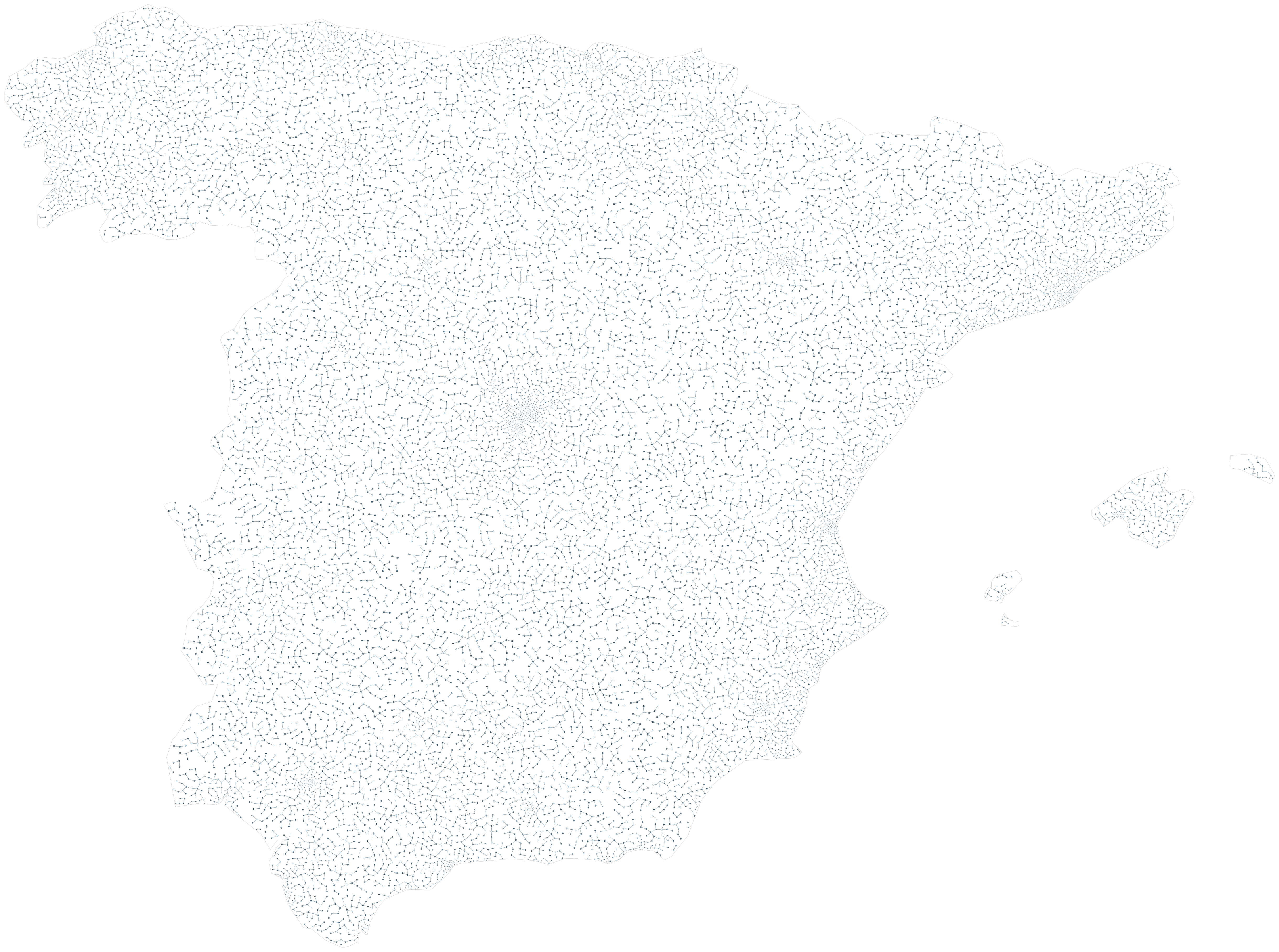
Spain: size and spacing / porcelain

graph-ics render --example spain_population --palette porcelain --output examples/output/spain_population-porcelain.png

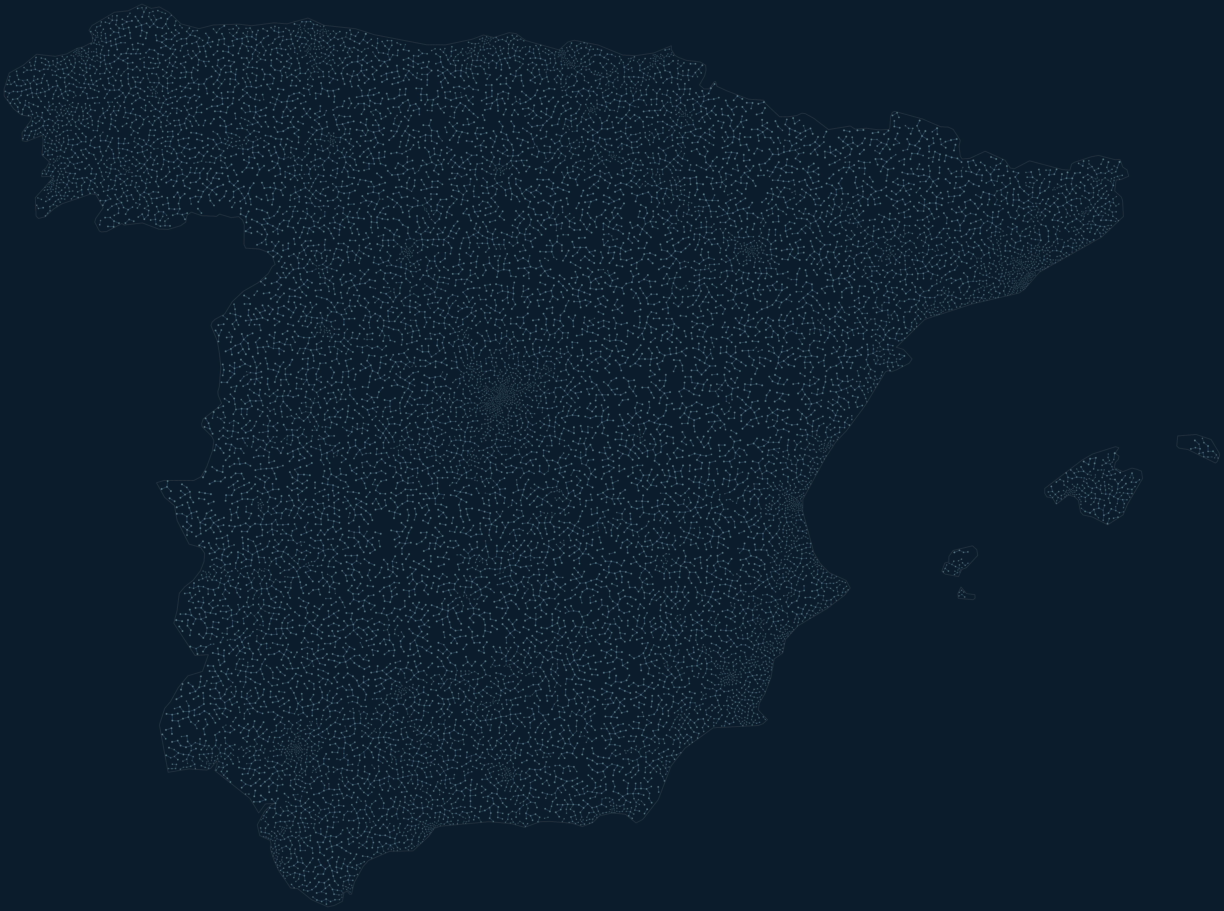
Spain: size and spacing / arctic

graph-ics render --example spain_population --palette arctic --output examples/output/spain_population-arctic.png

Spain uses the same 2020 WorldPop source and Natural Earth boundaries. The crop includes mainland Spain and the Balearic Islands; the Canary Islands are excluded. Small territories may be empty after geometric filtering.

Sources

WorldPop / CIESIN, Global High Resolution Population Denominators, 2020 density estimates, distributed under CC BY 4.0. Boundary: Natural Earth 5.1.2, public domain.

Download query and provenance

{
  "year": 2020,
  "units": "persons per square kilometre",
  "accessed": "2026-10-23",
  "raster_source": "https://worldpop.arcgis.com/arcgis/rest/services/WorldPop_Population_Density_1km/ImageServer",
  "raster_query": "https://worldpop.arcgis.com/arcgis/rest/services/WorldPop_Population_Density_1km/ImageServer/exportImage?f=json&bbox=-8.7%2C49.8%2C2.1%2C61.1&bboxSR=4326&imageSR=4326&size=360%2C560&format=tiff&pixelType=F32&interpolation=RSP_BilinearInterpolation&time=1577836800000&adjustAspectRatio=false&renderingRule=%7B%22rasterFunction%22%3A+%22None%22%7D",
  "raster_sha256": "1d2b1c05badd6fb27cd552efe0997db428d4b8649ee1ca806c1769f4ada6ab00",
  "boundary_source": "https://raw.githubusercontent.com/nvkelso/natural-earth-vector/v5.1.2/geojson/ne_50m_admin_0_countries.geojson",
  "boundary_sha256": "3e458fc036ad0a66411f2c1e6cac49c5d7bfb81cb1123bc513b22511a2b7fdeb",
  "raster_license": "CC BY 4.0",
  "boundary_license": "Public domain",
  "bbox": [-8.7, 49.8, 2.1, 61.1],
  "dimensions": [360, 560],
  "extent": {
    "xmin": -8.7,
    "ymin": 49.8,
    "xmax": 2.1,
    "ymax": 61.1,
    "spatialReference": {
      "wkid": 4326,
      "latestWkid": 4326
    }
  },
  "note": "Bilinear resampling of 1-km estimates to an educational grid; not population totals. Simplified Natural Earth 5.1.2 boundary."
}

Sources, licensing and transformations